I’m thrilled to share my submission for the Summer of Math Exposition! This essay is a nine-day diary of rediscovering Arnold’s topological proof. Before the diary begins: this problem stumped mathematicians like Euler, Bézout, and Lagrange for more than 200 years, and when it was finally solved, the reason turned out to be stranger than the theorem itself. Arnold found a proof that never touches Galois theory. It works by moving the roots of the polynomial around each other in a specific way — and the specific way turns out to be the entire secret. I didn’t invent this proof, but it took me nine days to make it mine, and I’ve tried to write it so that you don’t need a semester of abstract algebra to make it yours too.

Contents

• Day One — Why the theorem is important
• Day Two — Taking stock
• Day Three — Why n=5 is different
• Day Four — Radical depth 0
• Day Five — Radical depth 1
• Day Six — Radical depth 2
• Day Seven — Topological proof is more powerful
• Day Eight — My contribution
• Day Nine — Arnold’s insight

Day One — The Tempest

The storm arrived in the night. By morning, heavy rain was sheeting sideways across Tannsjö lake, and the pines were groaning under the gale. There was no question of going outside.

I sat in our guest cottage — ten square meters I built myself, just a desk, a chair, and a bunk bed — with a cup of coffee and a problem I had been carrying for years.

The Abel–Ruffini theorem. The fact that there is no formula in radicals for the roots of a general fifth-degree equation. Ruffini and Abel had proved it. Then Galois had illuminated it entirely with his theory of groups.

I had never read their proofs. Sitting there with the storm hammering the walls, I found myself thinking about the history of this problem rather than its solution.

Two hundred and fifty years. That is how long it took mathematicians to prove this theorem. Euler tried and could not do it. Bezout tried. Lagrange tried. Every major mathematician of the eighteenth century looked at the quintic and turned away. The problem resisted giants.

When Ruffini finally produced a proof — imperfect, contested — and Abel completed it, something shifted permanently in mathematics. Before Abel and Galois, the most prestigious and active part of mathematics was analysis — calculus, differential equations, and the mathematics of continuous change, the mathematics of Newton and Leibniz and their heirs.

The fact that the quintic resisted formula was striking enough. But the reason it resisted proved even more interesting. Galois found that reason, by inventing what we now call group theory. He saw that the solvability of an equation was governed by the symmetries among its roots, and that those symmetries formed a structure obeying its own laws. After Galois, algebra became as important to mathematical inquiry as analysis.

The idea was contagious. Sophus Lie, inspired by Galois, asked the analogous question for differential equations and was led to continuous groups — what we now call Lie groups. Decades later Emmy Noether proved that every continuous symmetry of a physical system corresponds to a conservation law, planting Lie’s machinery in the foundations of physics. From there the line runs through gauge theory to the Standard Model, whose entire architecture is the representation theory of Lie groups.

None of this would have unfolded the way it did without the quintic. It is the place where mathematics first learned to speak about symmetry as an algebraic structure.

Sitting in my ten square meters with the cold storm outside and a cup of hot coffee, I decided that I wanted to prove this theorem myself.

The reason I thought I had a chance was Vladimir Arnold. He had proven the theorem topologically rather than algebraically. The algebraic route meant wading through a thick textbook of preliminary theory — fields, extensions, solvable groups — and when the quintic finally arrived at the end, it was usually glossed over. That had never felt worth the trip. Topology was a different game. I looked at Arnold’s paper and did not understand it — but I got the basic idea.

That was enough. I did not know how long it would take. I did not know if I would succeed.

Day Two — The Drenching Drizzle

The fierce winds died overnight. The rain remained — steady, heavy, unhurried — and the sky settled into an unbroken slate gray. The streams ran dark with peat water. The forest was silent except for the soft percussion of rain on pine needles.

A good day for taking stock.

Before attempting to prove something impossible, it is worth being precise about what you know. I sat at my desk and laid out my tools.

The polynomial equation of degree $n$ is expressed with $n$ complex coefficients $c_1, \dots, c_n$.

I knew the Fundamental Theorem of Algebra: Every polynomial of degree $n$ has exactly $n$ roots in the complex numbers. That allows us to express the polynomial equation with $n$ complex roots $z_1, \dots, z_n$.

Multiplying the right hand side and identifying the coefficients leads to Vieta’s formulas.

$$
\begin{aligned}
c_1 &= -(z_1 + \dots + z_n) \\
c_2 &= z_1 z_2 + \dots + z_{n-1} z_n \\
\vdots \\
c_n &= (-1)^n z_1 \cdots z_n
\end{aligned}
$$

The sum of the roots gives one coefficient. The sum of all pairwise products gives another. All the way down to the product of all roots. This is not a minor bookkeeping fact — it is the bridge between two worlds. The roots live in one place; the coefficients live in another; Vieta’s formulas connect them with iron chains.

Here are some important observations.

1. A permutation of the roots does not change the coefficients.
2. In fact the permutations of the roots form a group under composition. What is striking about this operation is that it is not always commutative: applying permutation $a$ followed by $b$ does not always give the same result as $b$ followed by $a$. Lagrange had earlier introduced the idea of permuting roots. Ruffini was the first to sense that the structure of these permutation groups was what ultimately blocked a formula in radicals for the quintic. Cauchy later gave the first systematic study of permutations as algebraic objects.
3. Having the roots we can easily calculate the coefficients. But having the coefficients does not allow us to easily calculate the roots. In fact we need to find a formula that will allow us to do so, and finding such a formula is not easy as the history shows. In one direction it is easy, in the other direction it is hard.
4. Finding formulas means to find expressions of the type

$$
\begin{aligned}
z_1 &= f_1(c_1, \dots, c_n) \\
&\vdots \\
z_n &= f_n(c_1, \dots, c_n)
\end{aligned}
$$

The allowed formulas are allowed only to use the 4 arithmetic operations: addition, subtraction, multiplication, division, and the radicals. Other operations are not allowed.

Glancing outside, I watched rain trickle down the leaves of the large rhododendron bush, its purple buds waiting to burst.

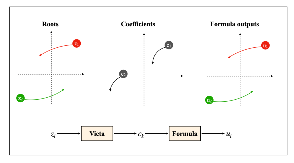
Figure 1: The three planes. When I move the roots the coefficients and the formula values move.

5. There are three main players in this theater. The roots, the coefficients and the formulas. And all of them deal with complex numbers. I began to think in terms of three complex planes.

The first is the root plane: this is where the $n$ roots of the polynomial live as points. I can move them freely and continuously. That insight came from Arnold.

The second is the coefficient plane: this is where the coefficients live. But the coefficients are not free. When the roots move, Vieta’s formulas drag the coefficients along automatically. They have no choice.

The third is the formula plane: It takes the coefficients as inputs and produces values claiming to be roots. When the coefficients move, the formula values move with them — again automatically, governed entirely by the formula’s algebraic structure.

I control the root plane. The formula controls nothing. It only reacts. Move the roots, and everything else follows by compulsion — Vieta compels the coefficients, and the formula compels its own values.

6. When I move the roots, the formula values must track the roots exactly. If the formula doesn’t do that then that formula is wrong. Because then I have found some roots for which the formula gives the wrong answer.

I lay down on my bunk bed and closed my eyes. I could hear the rain hitting the roof. I imagined moving the roots in complicated ways and I saw the formula values trying to track the roots. Given a formula could I move the roots so that the formula could not track them?

The rain became heavier and the sound on the roof became louder.

If I moved the roots through a sequence of twists that ended in a non-trivial permutation, the roots would swap places. But because the coefficients are blind to permutations, the coefficients would trace a path that ended exactly where it began — a closed loop. If the coefficients traveled in a loop, the formula, depending only on those coefficients, should also return to its starting point, that is make a loop. But since my roots did not make a loop, I would have a contradiction.

Unless, of course, the formula uses its radicals to break the loop. Radicals can split a closed path into an open one. For instance look at a circle around the origin in the complex plane. Its square root only traces a half circle ($\pi$ arc), failing to close.

My goal was suddenly clear and I got that idea from Arnold: I had to engineer special moves for the roots. A set of paths such that they would render the radicals utterly harmless, preventing them from splitting the loops. If I could find such magic paths I would be done.

I stood up. My brain was spinning. Enough for today.

Day Three — The Rising Mist

The rain stopped before dawn. I woke to silence and to mist — hanging over the lake, invading the land, wrapping around every tree trunk. The air smelled of pine and damp earth. The forest held its breath.

Yesterday two observations had stood out. One was topological: the possibility of moving the roots continuously. The other was algebraic: that permutations of roots are not always commutative. I had a feeling that this non-commutativity might be what made the quintic different. So for today I decided to set the topology aside and follow the algebraic thread instead. I wanted to see whether the degree of non-commutativity could explain the difference.

How do you measure the extent to which a group is non-commutative?

Two elements commute if $ab = ba$. Or equivalently, $aba^{-1}b^{-1} = e$, where $e$ is the identity element. So the elements do not commute if $aba^{-1}b^{-1} \neq e$. One measure is to take all elements of the group, multiply them against all other elements, and collect the results. That collection is called the commutator subgroup¹. Then repeat the process on the commutator subgroup. And again. And keep going until it eventually collapses to unity. The number of steps you have to do before it collapses to unity would be the measure of how non-commutative the group was.

So if we take $n=2$ we have 2 elements — the identity and one transposition. They commute trivially. One step and we are at unity.

If we take $n=3$ we have 6 elements. One step gives us 3 elements. One more step gives us unity. Two steps are needed.

If we take $n=4$ we have 24 elements. Taking the commutator of 24 elements against 24 elements is 576 commutators to compute — not something to do by hand. So I wrote a program to do that.

Looking at the result, I saw that one step gives 12 elements. Then 4. Then unity. Three steps are needed.

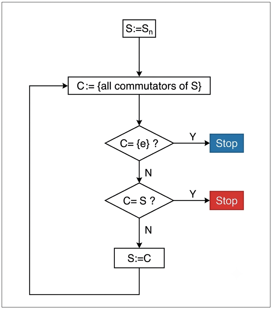
Figure 2: The commutator series of   can be calculated with a program. When I ran the program for n = 2, 3 and 4, the program stopped at blue stop (it reached the identity). But for n= 5  it stopped at the red stop (it never reached the identity).

For $n=5$ we have 120 elements. Taking the commutator of 120 elements against 120 elements is 14,400 commutators to compute — a huge job.

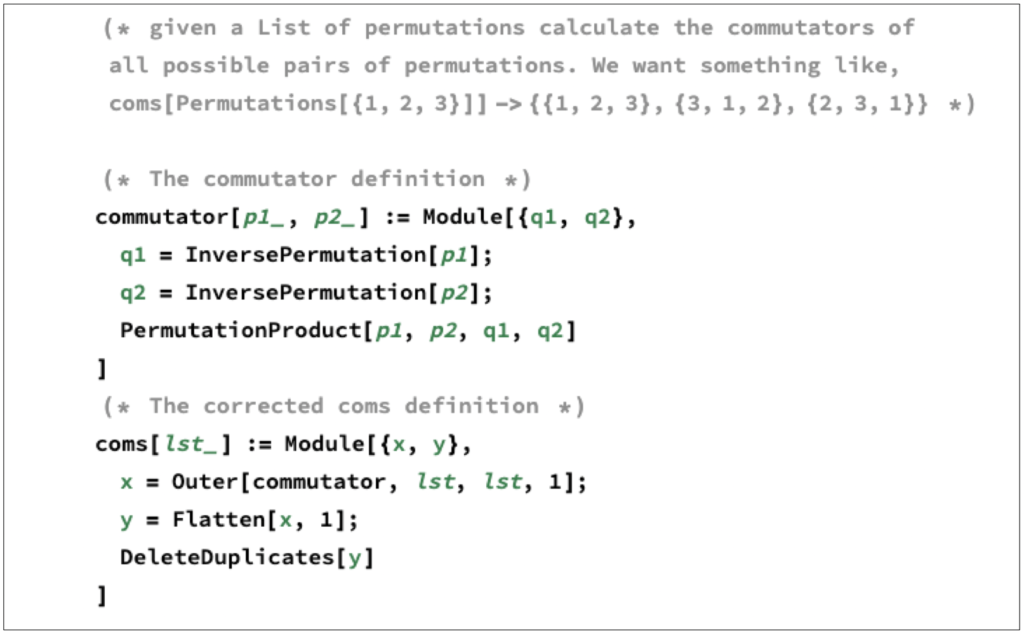
Figure 3: The commutator series of   can be calculated with this Mathematica program.

The program ran in seconds. One step gave 60 elements. The next step gave the same 60 elements back. So it would never end. I would never reach unity.

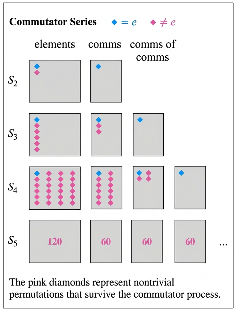
Figure 4: Commutator series

This was the aha moment.

This was the real reason why $n=5$ is fundamentally different. Of that I was sure, but I did not yet know why.

By afternoon the mist had lifted from the lake, but the clouds still covered the sky.

Day Four — Heavy Clouds

I was hoping for nice weather, but as I walked to the guest house, I noticed heavy, motionless clouds above. They pressed the forest in a tight box. The light was thin and diffused. Even the birds were silent.

I sat at my desk and thought about Arnold’s continuous root movements, about the non-trivial commutators, and about formulas having nested radicals. What do these have to do with each other, and how do I connect them to the proof of insolubility of the quintic?

I could see the goal — but not yet how to attack it. I have learned from experience that walking straight into a dense forest is how you lose a week, so before anything else I needed a plan.

I often think of Gelfand, who said that the number of ideas in mathematics is not large. Everything that is achieved comes from a few fundamental concepts, applied again and again with variation. So when you are stuck, the move is not to invent something new — it is to reach for one of the old, powerful tools and ask whether it fits here.

And one of the most powerful tools in all of mathematics is induction: prove the first simple case, then climb the ladder one rung at a time. My first instinct is always to look for that ladder. And there it was, sitting in the formulas — the radicals were nested, one inside another. I could start at the bottom, depth zero, no radicals at all, and climb one level, one more nested radical, at a time. I felt that this was the right road, even if I could not yet see the end of it.

Ok, so let’s start with a formula using no radicals. Choose a non-trivial permutation. Use Arnold’s idea, and instead of permuting the roots instantly, permute them using a continuous path (making sure that they avoid crossing each other, which is always possible² since we can choose different paths between start point and end point).

First, notice that a radical-free formula $f_i$ is single-valued and continuous in the coefficients. Because it claims to be a correct formula, at every instant its value has to be one of the roots — it is never allowed to drift off to something that is not a root³. At the start it equals root $i$. Now I move the roots continuously, keeping them apart from one another, which I can always arrange. Since the roots never touch and $f_i$ cannot jump from one to another, $f_i$ has no choice: it stays equal to root $i$ the whole time.

(A real formula would of course consist of several such expressions, one for each root. But the same reasoning applies independently to each of them, so it is enough to follow a single one.)

Since the coefficients are determined by the roots they have to move continuously as well. And since the coefficients are blind to root permutations, they must perform a loop.

I looked out the window and saw a robin with a rust-red breast, perched on a birch branch. It stretched its wings, glancing intently from side to side.

Now the formula values depend on the coefficients alone. And they are now using only the four arithmetic operations but no radicals. Does that guarantee that the formula values also track a loop?

Yes it does. Saying that a coefficient $c_i(t)$ makes a loop is the same as saying that $c_i(0) = c_i(1)$.

Now take a simple example. Let the function be $f(t) = c_1(t) + c_2(t)$. It moves in a loop because $f(0) = c_1(0) + c_2(0) = c_1(1) + c_2(1) = f(1)$. And that is true for the other three arithmetic operations – subtraction, multiplication and division⁴.

And for any combination of them, which the following example illustrates.

$$
f(t) = \frac{c_1(t) \, c_2(t) + c_3(t)}{c_4(t)}
$$

We see that $c_1(t) \cdot c_2(t)$ is a loop, let’s call it $d_1(t)$. So we can write:

$$
f(t) = \frac{d_1(t) + c_3(t)}{c_4(t)}
$$

Now $d_1(t) + c_3(t)$ is a loop, let’s call it $d_2(t)$. So we can write:

$$
f(t) = \frac{d_2(t)}{c_4(t)}
$$

Now $d_2(t) / c_4(t)$ is a loop, so $f(t)$ is a loop.

So I know that the roots perform a non-trivial permutation, that is they do not end up where they started. By the reasoning above the formula values perform a loop, that is they end up where they started. That is a contradiction since any correct formula must track the roots exactly, position by position, including the starting position and the ending position.

Of course the same argument works not only for the quintic ($n=5$), but also for the quadratic ($n=2$), the cubic ($n=3$), the quartic ($n=4$) as well. And indeed no radical-free formula exists for them either. But it does not work for the linear equation ($n=1$), because there is no non-trivial permutation in that case.

I had taken the first step, but something nagged at me. The argument I had just made — the loop, the contradiction — had not used the commutators at all. It ran exactly the same for the quadratic, the cubic, the quartic, the quintic; it did not care in the least that commutators for the quintic had refused to collapse.

The great discovery of Day Three, the one I felt was the key, had played no part whatsoever in the first step of the ladder. It was still sitting off to the side where I had left it, unexplained. Somewhere higher up the ladder it would have to come in — it had to, or the quintic would be no harder than the quadratic. But I could not yet see where. I took a deep breath. Tomorrow I will handle the case with one radical, and I wondered whether that was where the commutators would enter.

The clouds were thinning out, letting more light in. I heard a great tit chirp, do-da, do-da, do-da.

Day Five — Shifting Skies

The clouds fractured, and a cold wind from the north pushed them around. A gray, a white and sudden shocking blue. For a few minutes at a time, shafts of sunlight made the water droplets on the blueberry bushes glint like diamonds. Then another cloud, and the light was gone again.

I sat at my desk with a cup of coffee and yesterday’s loose thread in mind. The commutators had to be used somewhere. They were still waiting. Today I would climb one rung up the ladder — formulas with a single radical — and I had a quiet hope that this was where they would enter.

Today we are attacking formulas that have radicals, but no radicals within radicals. So the thing under the radical symbol, the radicand, is a radical-free expression, the thing we discussed yesterday.

So suppose we move the roots continuously⁵ so they end up in some non-trivial permutation. We will eventually have to choose this permutation carefully — that is where the work happens — but for now let’s just call it $p$ and see what it forces.

Each coefficient tracks a loop $A$. And each radicand tracks a loop $R$.

$$
p \to A \to R(A)
$$

Now our formula uses a radical $\sqrt[m]{R}$.⁶

Is it a loop?

If we can ensure that $\sqrt[m]{R}$ is a loop, then the same reasoning that ruled out a correct radical-free formula will also rule out this one.

Well $\sqrt[m]{R}$ is sometimes a loop but sometimes not. To see this, express the radicand in polar coordinates:

$$
R(t) = r(t), e^{i\theta(t)}
$$

Since $R$ is a loop, $R(0) = R(1)$:

$$
R(0) = R(1) = r(0), e^{i\theta(0)} = r(1), e^{i\theta(1)}
$$

which forces

$$
r(0) = r(1) \qquad \text{and} \qquad \theta(0) = \theta(1) + k \cdot 2\pi
$$

The integer $k$ is the winding number — how many times $R$ winds around the origin.

Taking the $m$-th root:

$$
\sqrt[m]{R(t)} = R(t)^{1/m} = r(t)^{1/m} \cdot e^{i\theta(t)/m}
$$

I looked out the window and, at first, thought the wind had died down; the leaves of the birches, oaks, and beeches had stopped moving. But the aspens told the truth — their leaves were still fluttering.

Now compare the endpoints. Substituting $\theta(0) = \theta(1) + 2\pi k$:

$$
\begin{aligned}
\sqrt[m]{R(0)} &= r(0)^{1/m} \cdot e^{i\theta(0)/m} \\
&= r(1)^{1/m} \cdot e^{i(\theta(1) + 2\pi k)/m} \\
&= r(1)^{1/m} \cdot e^{i\theta(1)/m} \cdot e^{i 2\pi k/m} \\
&= \sqrt[m]{R(1)} \cdot e^{i 2\pi k/m}
\end{aligned}
$$

So $\sqrt[m]{R(0)} = \sqrt[m]{R(1)}$ when $k = 0$, that is, when the radicand does not wind around the origin.

Here is the conclusion: If a radicand $R$ that tracks a loop never winds around the origin, then its radical $\sqrt[m]{R}$ will automatically track a loop.

We will call a loop that never winds around the origin, a harmless loop.

But how can we guarantee that our radicand never winds around the origin?

Ah here is where the commutator $p = [a,b] = aba^{-1}b^{-1}$ comes in. Look at what happens between the three planes:

$$
aba^{-1}b^{-1} \; \to \; ABA^{-1}B^{-1} \; \to \; R(A) R(B) R(A)^{-1} R(B)^{-1}
$$

(The notation above means “do this continuous move, then that one” — on the root plane, on the coefficient plane, and on the radicand plane alike.)

The commutator structure is preserved. ⁷

What is the winding number of our radicand commutator?

I leaned back. The sun had broken through and a sun ray hit me in the eyes. I had to squint. I looked at the lake. The surface flickered with a thousand tiny flashes.

If the winding number of $R(A)$ is $i$ and the winding number of $R(B)$ is $j$, then the total winding number is $i + j – i – j = 0$, because the winding number counts the net turning of the angle $\theta$ around the origin, so it adds when you concatenate paths and negates when you reverse them.⁸

So every radicand in our formula is harmless, which makes every radical in our formula track a loop. So we are now back in the situation we had yesterday. We have a rational expression of loops, so the whole formula tracks a loop. Which means that our formula values perform a trivial permutation.

And since our roots performed a non-trivial permutation, $aba^{-1}b^{-1}$, we conclude that the formula can’t be correct.

But why then does there exist a formula with one radical for the quadratic?

It’s because we require the existence of a non-trivial permutation $aba^{-1}b^{-1}$. For $n=3$ and higher there is such a non-trivial permutation. But for the quadratic there isn’t. (Recall Figure 2: for $n=2$ the commutator series collapses in a single step.) So the argument has nothing to bite on.

It’s worth noting that it rules out a radical depth-1 formula for the cubic and higher, which is consistent, since Cardano is depth 2 and Ferrari higher depth still.

So we have successfully attacked formulas with a radical of depth 1. But our formulas can have radicals within radicals.

Two days ago, I found that the commutator series for $n=5$ never terminates. Today I used one commutator to peel off one layer of radicals. I was beginning to sense the shape of the full argument: each level of the commutator series would peel off one more layer of nesting. For $n=5$, where the series never ends, I could keep peeling forever.

But let’s hurry slowly. Take one step at a time. So tomorrow we will attack formulas with nested radicals of depth 2.

I stepped outside. The cold north wind had dropped, and the lake had gone glass-still. A loon called from far down the shore — a note that carried across more water than it should. I crossed the mossy shore toward the tea-colored water. The air smelled of moss and layers of old pine needles pressed into the sodden earth.

Day Six — Spider’s Web

As I walked from the cottage to the guest house this morning, I noticed a spider’s web where there was none yesterday. It looked delicate and glowed white in the sunlight. A light breeze made it shiver, but it was safe; the web was much stronger than its thin threads let on. As I unlocked the guest house an irritating fly was buzzing around my head.

Let’s recollect then when we are talking about commutators we are only interested in non-trivial commutators, since otherwise the basic argument that the formula values can’t trace the roots, doesn’t hold.

Let’s study a formula with two nested radicals.

Let’s use $p = [a,b] = aba^{-1}b^{-1}$ to denote a commutator.

When I move the roots along a permutation each coefficient traces a loop (though not necessarily a harmless one).

1. What happens if I move the roots along the commutator $[a,b]$? The commutator zeros out each coefficient’s winding number, around any point of any continuous function of the coefficients, because winding numbers add under concatenation and negate under reversal. That makes every coefficient trace a harmless loop.

What happens with a radicand that contains a radical whose radicand is harmless?

As we said yesterday the inner radical (whose radicand is harmless) closes up into a loop. But that loop is not necessarily harmless. And that puts the inner radical on par with the coefficient loops.

So from this point on, the inner radical can be forgotten as a radical. It’s just another loop in the same category as the coefficient loops. Whatever trick worked on coefficients to make them harmless will now work on this loop too.

This is a key point, so let me repeat it: The inner radical is just another loop in the same category as the coefficient loops.

2. What happens along a commutator of commutators $[p,q]$, where $p = [a,b]$ and $q = [c,d]$? Each of $[a,b]$ and $[c,d]$ already makes the inner radical close into a loop. The outer commutator $[p,q]$ then plays the same trick one level up: it forces the coefficient loops and the inner-radical loop to all be harmless. The outer radicand, that is built from these, is then harmless, and the outer radical closes into a loop of its own.

And we can apply this reasoning to any depth of radicals.

A commutator prevents a radical from breaking the loop. But a commutator of commutators (denoted commutator$^2$) prevents a nested radical of depth 2 to break the loop. And a commutator$^k$ prevents a radical of depth $k$ to break the loop.

And that explains why nothing here forbids a formula for $n = 2, 3$, and $4$. ⁹

The $n=2$ lacks a non-trivial commutator. So a formula with one radical is possible.

The $n=3$ lacks a non-trivial commutator$^2$, so a formula with radical depth 2 is possible.

The $n=4$ lacks a non-trivial commutator$^3$, so a formula with radical depth 3 is possible.

But $n=5$ has a non-trivial commutator$^k$, for any $k$, so no formula with radical depth $k$ is possible.

So there it is:

That proves the theorem: There is no formula in radicals that expresses the roots of a general polynomial of degree $n \geq 5$ in terms of its coefficients.

And here, at last, is where Day Three pays off. To defeat a formula of depth $k$, I need a single root-move that is a nontrivial permutation and at the same time a commutator$^k$ — and whether such a move exists is precisely the thing my program measured on day 3. The collected commutators, then the commutators of those, and so on, are nothing but the rungs of the commutator series. So “a nontrivial commutator$^k$ exists” and “the series has not yet collapsed to unity by step $k$” are not two facts but one and the same.

As I walked back to the cottage I saw a fly in the spider’s web. It was wrapped in a cocoon and did not move.

Day Seven — The Clearing

By morning the lake was still. The mist was gone. For the first time in days the sky was an unbroken blue, and the pines stood sharp against it.

I’ve shown that the coefficients trace a harmless loop when constructed with commutators of type $ABA^{-1}B^{-1}$. But the radicand is some function $R(c_1, c_2, \dots)$ of the coefficients. As the coefficients trace a loop of type $ABA^{-1}B^{-1}$, the radicand traces some loop $\Gamma$ in $\mathbb{C}$. Is $\Gamma$ necessarily a harmless loop?

Yes — the radicand is some function $R(c_1, c_2, \dots)$ of the coefficients. But not any function. It is a function that only uses arithmetic operations (plus, minus, multiplication and division).

Remember when roots perform $aba^{-1}b^{-1}$ the coefficients perform $ABA^{-1}B^{-1}$. The paths $a$ and $b$ are permutation paths. $aba^{-1}b^{-1}$ is also a permutation path. $A$ and $B$ are loops. $ABA^{-1}B^{-1}$ is a harmless loop.

We are talking about three layers: roots, then coefficients, then radicand. When the roots walk backward ($a^{-1}$), the coefficients also walk backward ($A^{-1}$).

Think about the radicand, not as a sum of separate coefficient pieces, but as a single number that depends on wherever the coefficients happen to be at each moment. As the coefficients walk forward along path $A$, the radicand traces out some path of its own. When the coefficients later walk backward along that same path $A$, undoing their steps exactly, the radicand must retrace its own path exactly in reverse. There’s no way around this: the radicand only depends on where the coefficients are, so if the coefficients are reversing their steps, the radicand is reversing its steps too, frame for frame.

Nothing in the argument actually cares that I am using plus, minus, times, and divide. All it needs is that the radicand, at every instant, is continuous and single-valued. So if I let my formula use functions like sine, or the exponential function, alongside the arithmetic operations, the same argument would still hold, word for word.

However the functions like $\ln(z)$ and $\sqrt{z}$ are multivalued and the argument above cannot be applied.

Theta functions $\theta(z, \tau)$ can solve quintics as proved by Hermite. But they are not just functions of $z$, but of $\tau$ as well. In fact they are modular forms in $\tau$, but that’s another discussion.

So Arnold’s topological proof is more powerful than conventional Galois theory in that it shows that the polynomial equations of order $n \geq 5$ not only fail to have a solution in terms of the arithmetic operations and radicals but also when including continuous single-valued functions like the exponential function and the sine function.

I went outside. The lake was flat and bright. I walked to the water’s edge. A group of water striders skated across the surface, casting sharp shadows on the lake bed. A lonely strider was standing still, dreaming in the sun.

Day Eight — The Calm

The lake was mirror-flat. The storm felt like something from another life. I sat on the dock and dangled my legs with my feet in the water.

I had proved nothing new. The theorem was settled in the nineteenth century, by Ruffini and Abel. I knew it when I sat down on day one with the storm hammering the walls.

And yet it felt like something genuine. Not discovery — something quieter than that. Understanding from inside, rather than from outside. There is a difference between knowing that a proof exists and having walked through it yourself, made the turns yourself, felt where it resists and where it opens. The map is not the walk.

Moving the roots felt natural, because the roots are what I control and permute. The coefficients follow. The formula only reacts. Starting from the roots puts me where my intuition lives, before the abstraction begins.

Arnold used technical terms like monodromy, solvable group, derived subgroup, braid group, homomorphism, branched coverings, etc. They are correct, but if a reader is unfamiliar with them, they might feel like closed doors. I avoided all that. And that I think makes the proof more accessible to newcomers.

I introduced language that Arnold didn’t use. Harmless loops. The three spaces. The moment when the inner radical gets promoted to the same category as coefficient loops and can be forgotten as a radical. These are doors that open gently, and invite the reader.

However I also want to acknowledge that Arnold’s terminology is good — precise names for precise structures. Arnold’s terms are right for people who need them, and mine are right for people who don’t need them yet.

I spent several days trying to understand the proof. My effort has no value an accountant would recognize. But the question had caught me. What was it that made this proof so difficult — that took two hundred and fifty years, that turned away Euler and Lagrange, that finally changed the way we think about mathematics and science? I wanted to know. Not to be told. To let my own mind walk the strange path and understand.

I do not claim or aim in this essay to provide a rigorous proof, even though I tried to address some of the technical issues. Rigor, when applied too early, can obscure the shape of a proof. That is why I could not understand Arnold’s version, and why I had to build my own.

Beneath a brilliant, high-hanging sun, the lake glittered. Fifty meters out, a solitary heron paced the shoreline of a small island, completely unaware of me and the quintic.

Day Nine — New Storm Coming

A heavy thud on the guest house window. I went outside and found a jay lying dead on the moss. Above the trees the clouds were piling up — not the small soft ones, but the tall columns that climb toward the sky. I went back inside.

I thought about Arnold and how he came up with his proof. What was the main insight he had that others before him did not?

He knew that each permutation did nothing to the coefficients (they were blind to permutations). And he knew that the formulas depended only on coefficients. So when you make a permutation the coefficients stay put. So the formula values that only depend on the coefficients should also stay put.

So the formula values are drawn by the two forces when the roots make a permutation.

1. Since coefficients don’t flip, the formula values should not either.
2. The requirement is that the formula values reproduce the roots. Otherwise the formula is not correct.

He knew that radicals are multivalued and that was what made the trick above possible. For n = 2, 3 and 4 radicals could make the trick but not for n = 5.

But Arnold didn’t have the control of which branch the radicals would choose. And then it must have hit him.

He could force the radical to choose only one branch, if he chose to permute the roots, not by an instant switch, but by a continuous movement.

That was the aha moment. The move that made everything possible.

Once equipped with this idea, I was able to make my own proof during 8 days. But I got this idea from Arnold, and without this idea I would be stuck like everyone else.

Before Arnold, the unstated assumption was that permutations are instantaneous swaps. Arnold made them continuous motions. And if you think about how permutations actually happen in the physical world — two objects exchanging places — the motion is continuous.

The culprit is the silent assumption. A prejudice, if you like. And it often takes a genius to see that the assumption was never true — and that letting go of it is not a loss but an opening. Breakthroughs often come from questioning hidden assumptions. (In Arnold’s case, that permutations are instantaneous).

I looked out the window and saw the jay standing on shaky legs. He wasn’t dead. He spread his wings, and was gone.

Footnotes

1. Pedantic note: the commutator subgroup is the subgroup generated by commutators, and in general the raw set of commutators is not closed under products. In Sₙ and Aₙ, happily, every element of the derived subgroup is itself a commutator, so my program’s raw set coincides with the subgroup and no closure step is needed. ↩︎
2. Take the case of $n=2$. It is obvious that you can move from $z_1$ to $z_2$, and at the same time move from $z_2$ to $z_1$. Just pick a line between them and let the first path go above the line and the second go below it. And since any permutation can be done as a series of such transpositions, one after another in series, it should be obvious that collisions can be avoided. ↩︎
3. Why at every instant? Because the moving coefficients at each moment define a perfectly ordinary polynomial, and a general formula must deliver a root for every polynomial — not just our starting one. If at some instant the formula’s value were not a root, we would have found coefficients where the formula fails. (For formulas with radicals, one must also check that the value we track stays on a branch that makes the formula correct. The key is that correctness at a single point could be a coincidence — even a wrong branch can accidentally hit a root — but correctness on a whole neighborhood of coefficient values cannot, and a correct formula, having only finitely many branches, must have at least one branch that is correct on a full neighborhood of our start. That branch’s correctness is an identity, not a coincidence, and an identity survives the journey: by continuity it cannot fail at an isolated instant without failing on the way there (footnote 4). We track that branch.) ↩︎
4. Since we are dealing with division, we must prevent any denominator from becoming zero. We can always do this: we perturb the path of the roots so that the resulting coefficient path avoids bad points where a denominator vanishes (the bad set has measure zero).
   Imagine a path in the complex plane from $z_{\text{start}}$ to $z_{\text{end}}$, and suppose it crosses a finite number of bad points — places where a denominator vanishes. We can always find another path from $z_{\text{start}}$ to $z_{\text{end}}$ that avoids every one of them. The reason is geometric: the complex plane has two real dimensions, so removing finitely many points leaves it still connected. There is always room to go around.
   Since the bad set has measure zero, a generic perturbation can always be made to avoid it. (For the formal statement, see Needham, Visual Complex Analysis, §2.2 Topological Properties of the Complex Plane.) ↩︎
5. A word on the logical order before we proceed, because it’s easy to get backwards. We do not first pick a permutation and then check what formulas it rules out. We do it the other way around. A would-be formula is handed to us, with all of its structure already fixed — in particular its radical depth $k$. Only then do we go looking for a root-move that breaks it: a move that produces a non-trivial permutation and, at the same time, forces every radical at every level to close into a loop. The depth $k$ of the formula is what tells us how deep the commutator nesting in our root-move needs to be. The formula commits first, and we respond. The question is not “is there a single root-move that defeats every formula at once?” — that would be a much harder and unnecessary claim — but “for every formula of depth $k$, is there some root-move, tailored to it, that defeats it?” ↩︎
6. A possible source of confusion: one might think the multi-valuedness of the radicals matters here. It does not. The $m$-th root of a complex number is, in principle, multi-valued — there are $m$ possible choices for it. But in our setting that ambiguity disappears. At $t=0$ the formula equals a specific root, and that fixes one specific value for $\sqrt[m]{R}$ at $t=0$. From there, continuity takes over: as $R$ moves, $\sqrt[m]{R}$ must move continuously along with it, never jumping from one branch to another. So at every instant $\sqrt[m]{R}$ is a single, well-defined number. The only question is whether, after $R$ has completed its loop, $\sqrt[m]{R}$ has come back to where it started. ↩︎
7. Why does the commutator pattern survive the trip? Because the only thing I am using about these maps — roots to coefficients, then coefficients to radicand — is that each value depends only on where the thing it follows currently sits. Nothing else. So if I run move $a$ and then move $b$ on the roots, the coefficients have no choice but to run $A$ and then $B$, and the radicand to run $R(A)$ and then $R(B)$: doing one move after another above produces the matching moves, in the same order, below. Reversal works the same way — when the roots retrace $a^{-1}$, the coefficients retrace $A^{-1}$ and the radicand retraces $R(A)^{-1}$, step for step. Concatenation carries through as concatenation and reversal as reversal, so the whole pattern $aba^{-1}b^{-1}$ arrives intact as $ABA^{-1}B^{-1}$ and then as $R(A)R(B)R(A)^{-1}R(B)^{-1}$. That is all I mean by saying the commutator structure is preserved. ↩︎
8. There is one potential issue: what if the radicand $R$ passes through zero? The winding number of $R$ is only defined if $R$ never vanishes — if it hits the origin, the angle $\theta$ is undefined and the whole polar argument breaks down. But this is the same type of problem we met yesterday when discussing denominators, and it is handled in the same way. The set of coefficient values for which $R=0$ has measure zero in coefficient space. Since we are free to choose how we move the roots — we can always perturb the root paths so that the coefficient paths miss every point where $R$ vanishes. ↩︎
9. Showing that the obstruction runs out is not the same as building a formula. The fact that Cardano and Ferrari actually found them is separate work. I have only shown why my argument has nothing left to say against them. ↩︎